extractMoor

Another key functionality of the remora package allows users to integrate acoustic telemetry data with physical and biological parameters collected on the IMOS National Mooring Network. The National Mooring Network is a collection of mooring arrays strategically positioned in Australian coastal waters that includes regional arrays of shelf moorings, acidification moorings, acoustic observatories and a network of National Reference Stations. This package allows the user to match environmental data collected from these mooring stations to each tag detection. Associating environmental data to detections provides a means to analyse environmental or habitat drivers of occurrence, presence and movement of animal monitored using acoustic telemetry.

We advocate for users to first undertake a quality control step using the runQC() function and workflow before further analysis (see vignette('runQC')), however the functionality to append environmental data will work on any dataset that has at the minimum spatial coordinates and a timestamp for each detection event. Currently, the focus of this package is to integrate animal telemetry data and environmental data housed within the Integrated Marine Observing System, and therefore primarily focuses within Australia. As this package develops, more sources of environmental data will be added to allow for users to access more datasets across Australia and globally.

Types of environmental data

This package allows users to access a range of ocean datasets that have undergone a quality control process and housed within the Integrated Marine Observing System database and can also be explored through the Australian Ocean Data Network portal. There are primarily two types of environmental data that users can currently access:

1. Remote sensed environmental data

2. In-situ environmental data from moorings at fixed locations

The imos_variables() function will help the user identify currently available environmental layers that can be accessed and associated. Variables include spatial layers including bathy and dist_to_land, which provide distance measures of bathymetry (in meters) and proximity to land (in kilometers). Variable names that start with rs_ are remote sensed environmental layers, and variables starting with moor_ include in-situ environmental layers.

library(tidyverse)
library(remora)

imos_variables()

Variable	Platform	Temporal resolution	Units	Function to use	Description	Source
bathy	Composite raster product		meters	extractEnv()	Australian Bathymetry and Topography Grid. 250 m resolution.	Geosciences Australia
dist_to_land	Raster product		kilometers	extractEnv()	Distance from nearest shoreline (in km). Derived from the high-resolution Open Street Map shoreline product.	This package
rs_sst	Satellite-derived raster product	daily (2002-07-04 - present)	degrees Celcius	extractEnv()	1-day multi-swath multi-sensor (L3S) remotely sensed sea surface temperature (degrees Celcius) at 2 km resolution. Derived from the Group for High Resolution Sea Surface Temperature (GHRSST)	IMOS
rs_sst_interpolated	Raster product	daily (2006-06-12 - present)	degrees Celcius	extractEnv()	1-day interpolated remotely sensed sea surface temperature (degrees Celcius) at 9 km resolution. Derived from the Regional Australian Multi-Sensor Sea surface temperature Analysis (RAMSSA, Beggs et al. 2010) system as part of the BLUElink Ocean Forecasting Australia project	IMOS
rs_chl	Satellite-derived raster product	daily (2002-07-04 - present)	mg.m-3	extractEnv()	Remotely sensed chlorophyll-a concentration (OC3 model). Derived from the MODIS Aqua satellite mission. Multi-spectral measurements are used to infer the concentration of chlorophyll-a, most typically due to phytoplankton, present in the water (mg.m-3).	IMOS
rs_current	Composite raster product	daily (1993-01-01 - present)	ms-1; degrees	extractEnv()	Gridded (adjusted) sea level anomaly (GSLA), surface geostrophic velocity in the east-west (UCUR) and north-south (VCUR) directions for the Australasian region derived from the IMOS Ocean Current project. Two additional variables are calculated: surface current velocity (ms-1) and bearing (degrees).	IMOS
rs_salinity	Satellite-derived raster product	weekly (2011-08-25 - 2015-06-07)	psu	extractEnv()	7-day composite remotely sensed salinity. Derived from the NASA Aquarius satellite mission (psu).	IMOS
rs_turbidity	Satellite-derived raster product	daily (2002-07-04 - present)	m-1	extractEnv()	Diffuse attenuation coefficient at 490 nm (K490) indicates the turbidity of the water column (m-1). The value of K490 represents the rate which light at 490 nm is attenuated with depth. For example a K490 of 0.1/meter means that light intensity will be reduced one natural log within 10 meters of water. Thus, for a K490 of 0.1, one attenuation length is 10 meters. Higher K490 value means smaller attenuation depth, and lower clarity of ocean water.	IMOS
rs_npp	Satellite-derived raster product	daily (2002-07-04 - present)	mgC.m_2.day-1	extractEnv()	Net primary productivity (OC3 model and Eppley-VGPM algorithm). Modelled product used to compute an estimate of the Net Primary Productivity (NPP). The model used is based on the standard vertically generalised production model (VGPM). The VGPM is a “chlorophyll-based” model that estimates net primary production from chlorophyll using a temperature-dependent description of chlorophyll-specific photosynthetic efficiency. For the VGPM, net primary production is a function of chlorophyll, available light, and the photosynthetic efficiency. The only difference between the Standard VGPM and the Eppley-VGPM is the temperature-dependent description of photosynthetic efficiencies, with the Eppley approach using an exponential function to account for variation in photosynthetic efficiencies due to photoacclimation.	IMOS
moor_sea_temp	Fixed sub-surface moorings	hourly	degrees Celcius	extractMoor()	Depth-integrated in-situ, hourly time-series measurements of sea temperature (degrees Celcius) at fixed mooring locations	IMOS
moor_psal	Fixed sub-surface moorings	hourly	psu	extractMoor()	Depth-integrated in-situ, hourly time-series measurements of salinity (psu) at fixed mooring locations	IMOS
moor_ucur	Fixed sub-surface moorings	hourly	ms-1	extractMoor()	Depth-integrated in-situ, hourly time-series measurements of subsurface geostrophic current velocity in the east-west direction (ms-1) at fixed mooring locations	IMOS
moor_vcur	Fixed sub-surface moorings	hourly	ms-1	extractMoor()	Depth-integrated in-situ, hourly time-series measurements of subsurface geostrophic current velocity in the north-south direction (ms-1) at fixed mooring locations	IMOS
BRAN_temp	3D Raster product	daily (1993-01-01 - present)	degrees Celcius	extractBlue()	Water temperature at specified depth from the surface to 4,509-m depth	Bluelink (CSIRO)
BRAN_salt	3D Raster product	daily (1993-01-01 - present)	psu	extractBlue()	Water salinity at specified depth from the surface to 4,509-m depth	Bluelink (CSIRO)
BRAN_cur	3D Raster product	daily (1993-01-01 - present)	ms-1; degrees clockwise	extractBlue()	Geostrophic velocity in the east-west (UCUR) and north-south (VCUR) directions from the surface to 4,509-m depth. Two additional variables are calculated: BRAN_spd = current velocity (ms-1) and BRAN_dir = current bearing (degrees).	Bluelink (CSIRO)
BRAN_wcur	Raster product	daily (1993-01-01 - present)	ms-1	extractBlue()	Vertical current speed in the water column is calculated (negative = downwards; positive = upwards) using the layers available between the surface to 200-m depths.	Bluelink (CSIRO)
BRAN_ssh	Raster product	daily (1993-01-01 - present)	meters	extractBlue()	Sea surface height at the water surface	Bluelink (CSIRO)
BRAN_mld	Raster product	daily (1993-01-01 - present)	meters	extractBlue()	Mixed layer depth in relation to the water surface	Bluelink (CSIRO)
BRAN_wind	Raster product	daily (1993-01-01 - present)	ms-1; degrees clockwise	extractBlue()	Two variables are calculated, including BRAN_wind_spd = wind velocity (ms-1) and BRAN_wind_dir = wind bearing (degrees).	Bluelink (CSIRO)

In this vignette we will explore accessing and extracting in-situ data from the IMOS National Mooring Network. A suite of additional functions is also available to access enbvironmental data gatehred via remote sensing (see vignette('extractEnv')).

Usage of the `extractMoor()` function

Load example dataset

The primary function to extract and append in-situ data collected by the IMOS National Mooring Network to acoustic detection data is the extractMoor() function. Lets start with a dataset that has undergone quality control (see vignette('runQC')).

## Example dataset that has undergone quality control using the `runQC()` function
data("TownsvilleReefQC")

## Un-nest the output and retain detections flagged as 'valid' and 'likely valid' (Detection_QC 1 and 2)
qc_data <- TownsvilleReefQC %>% 
  tidyr::unnest(QC) %>% 
  dplyr::filter(Detection_QC %in% c(1,2))

Lets have a quick look at the spatial patterns in detection data for each tag deployment:

library(ggplot2)
library(ggspatial)

qc_data %>% 
  group_by(transmitter_id, station_name, installation_name, receiver_deployment_longitude, receiver_deployment_latitude) %>% 
  dplyr::summarise(num_det = n()) %>% 
  ggplot() +
  annotation_map_tile('cartolight') +
  geom_spatial_point(aes(x = receiver_deployment_longitude, 
                         y = receiver_deployment_latitude, 
                         size = num_det, 
                         color = installation_name), 
                     crs = 4326) +
  facet_wrap(~transmitter_id,nrow=3) +
  theme(legend.position="bottom")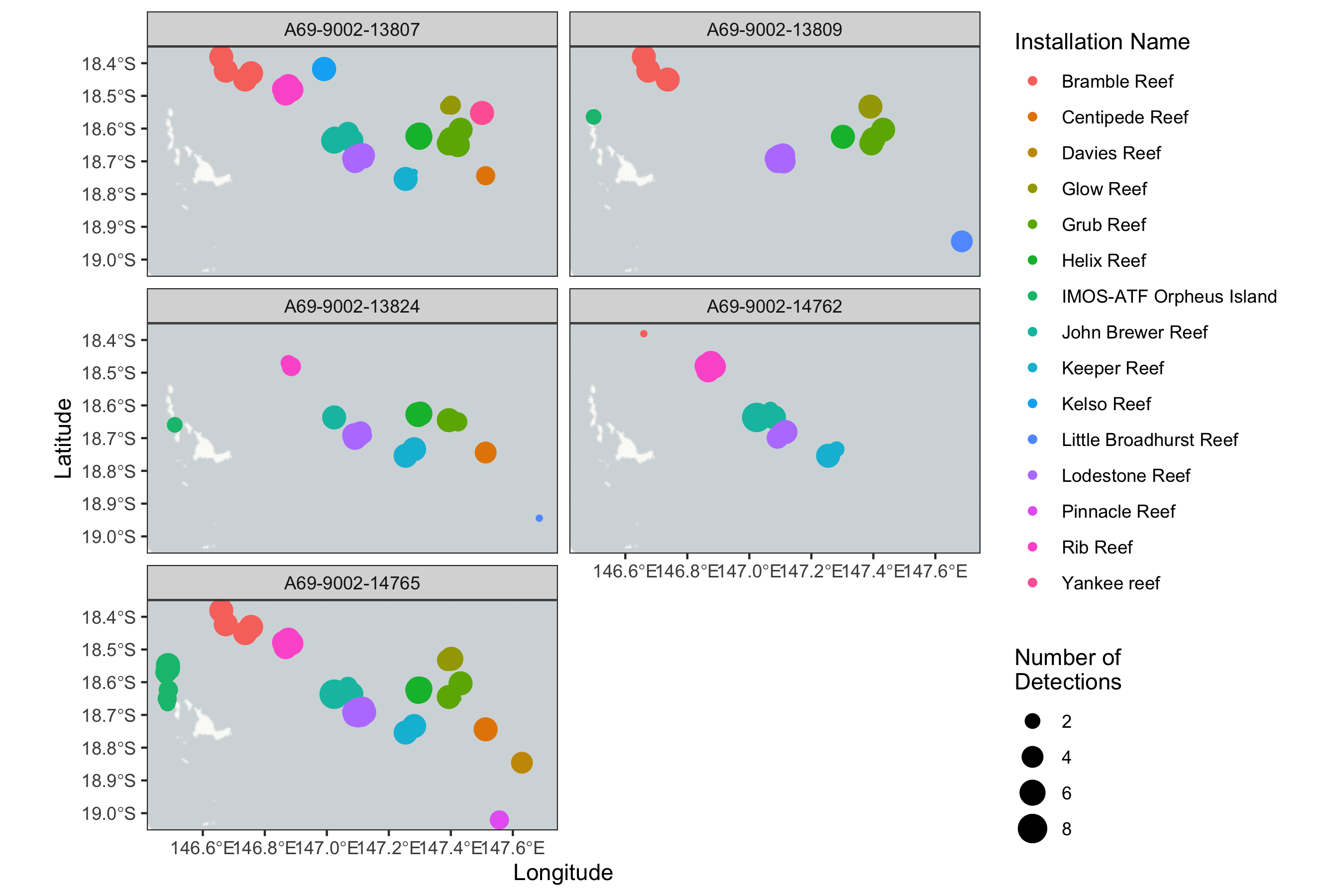

We can also have a look at the temporal pattern in detections:

qc_data %>% 
  mutate(date = as.Date(detection_datetime)) %>% 
  group_by(transmitter_id, date, installation_name) %>% 
  dplyr::summarise(num_det = n()) %>% 
  ggplot(aes(x = date, y = transmitter_id, color = installation_name, size = num_det)) +
  geom_point() +
  theme_bw()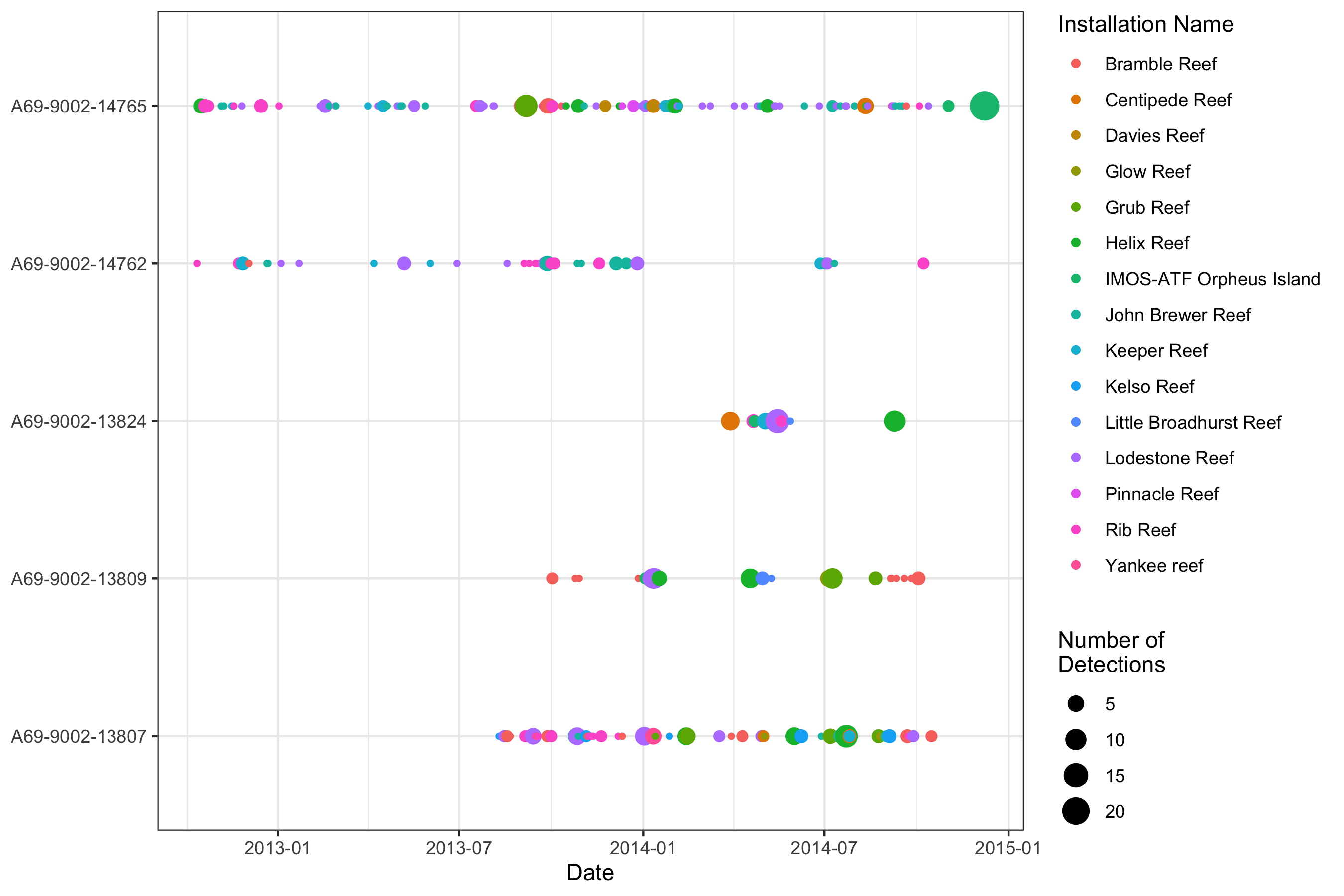

Moorings data source

Lets have a quick look at the spatial arrangement of the IMOS National Mooring Network.

In this example, we will identify and plot the location of moorings in Australian coastal waters which have records of sea water temperature

Each variable will need to be accessed one at a time using the mooringDownload() function. There is only one parameter within the function that can help the user identify the variable required:

sensorType: the name of the environmental variable to download and append. This can be temperature, velocity, salinity, oxygen.

# Generate a table containing IMOS moorings metadata for only those moorings with temperature data
moorT <- mooringTable(sensorType="temperature")

# PLot the location of the moorings with associated metadata
library(leaflet)
leaflet() %>%
  addProviderTiles("CartoDB.Positron") %>%
  addMarkers(lng = moorT$longitude, lat = moorT$latitude,
             popup = paste("Site code", moorT$site_code,"<br>",
                           "URL:", moorT$url, "<br>",
                           "Standard names:", moorT$standard_names, "<br>",
                           "Coverage start:", moorT$time_coverage_start, "<br>",
                           "Coverage end:", moorT$time_coverage_end))

Find closest mooring to our animal detections

To identify which is the appropriate mooring with which to append to our acoustic detections, we’ll run the getDistance() function. This function will assign the moor_site_code of the closest mooring to each tag detection, the straight line distance of the mooring to the receiver station location (closest_moor_km), along with the mooring’s temporal coverage (moor_coverage_start and moor_coverage_end), and whether or not the detection_datetime stamp falls within this coverage period (is.coverage = TRUE/FALSE).

In this function, the user specifies which detection dataset with which they which to merge with the available moorings data.

moorLocations: the dataframe containing the locations of the IMOS moorings generated using the mooringTable() function.
trackingData: the dataframe containing acoustic detection data in IMOS QC format

#Extract the nearest mooring to each station where a tag was detected
det_dist <- getDistance(trackingData = qc_data, 
                        moorLocations = moorT,
                        X = "receiver_deployment_longitude",
                        Y = "receiver_deployment_latitude",
                        datetime = "detection_datetime")

In order to identify which moorings do not have temporal coverage during the period when tag detections were obtained, we have provided the getOverlap() function. In this function, we simply enter the detection dataset (det_dist) which also contains the nearest moorings data generated using the above getDistance() function. What is returned is a table containing the proportion of tag detections that fell within the coverage period of the mooring deployment at which it was assigned: moor_site_code, moor_coverage_start and moor_coverage_end.

# Which moorings have overlapping data with detections?
mooring_overlap <- getOverlap(det_dist)
mooring_overlap

As Poverlap = 1 for all three moorings datasets, all our detections have temporal overlap with these mooring deployments. IF some of the moorings had partial/no coverage during the tag release period, we would consider dropping these from the moorT object before re-running the getDistance() function.

Let’s plot the spatial arrangement of these mooring stations on an interactive map with our tag detections at receiver stations.

# Filter for only those moorings which are closest to receivers and also have overlapping detection intervals
moorT_new <- moorT %>% 
  filter(site_code %in% mooring_overlap$moor_site_code)

#Summarise dataset so only a single row per receiver station
qs_stat <- qc_data %>% 
  group_by(station_name, installation_name, 
           receiver_deployment_longitude, 
           receiver_deployment_latitude) %>% 
  dplyr::summarise(num_det = n(),
            first_detection = min(detection_datetime),
            last_detection = max(detection_datetime))

# make palette for number of detections at stations
library(viridisLite)
domain <- range(qs_stat$num_det) # get domain of numeric data for colour scalse
pal <- colorNumeric(palette = viridis(100), domain = domain)

# Draw the map
leaflet() %>%
  addProviderTiles("CartoDB.Positron") %>%
  addMarkers(lng = moorT_new$longitude, lat = moorT_new$latitude, 
             popup = paste("Site code", moorT_new$site_code,"<br>",
                           "URL:", moorT_new$url, "<br>",
                           "Standard names:", moorT_new$standard_names, "<br>",
                           "Start:", moorT_new$time_coverage_start, "<br>",
                           "End:", moorT_new$time_coverage_end)) %>%
  addCircleMarkers(data=qs_stat,
                   lng = qs_stat$receiver_deployment_longitude, 
                   lat = qs_stat$receiver_deployment_latitude,
                   radius = 6,
                   color=~pal(num_det),
                   stroke=FALSE,
                   fillOpacity=0.5,
                   popup = paste("Station name", qs_stat$station_name,"<br>",
                                 "Installation name:", qs_stat$installation_name, "<br>",
                                 "Tag detections:", qs_stat$num_det, "<br>",
                                 "First tag detection:",qs_stat$first_detection, "<br>",
                                 "Last tag detection:",qs_stat$last_detection))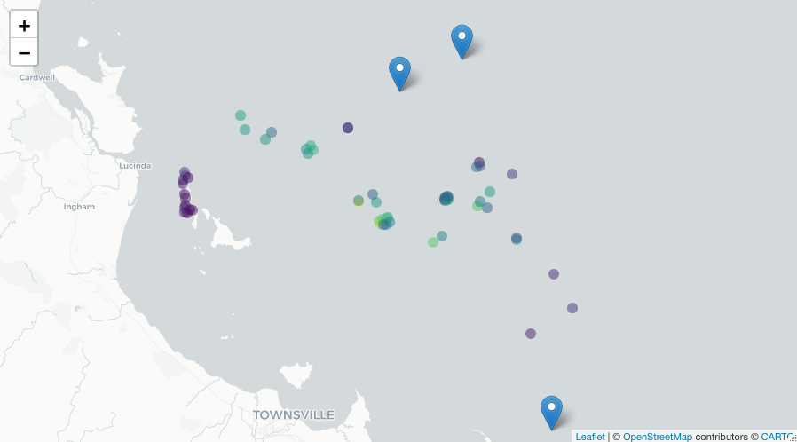

Moorings data download

Now that we have matched each animal detection with an appropriate moor_site_code, we will download the data time series for moorings derived water temperature for each mooring site code from the AODN Thredds file sever.

Although this function provides the capacity to download various sensor types (i.e. temperature, velocity, salinity or oxygen), each variable can only be accessed one at a time using the mooringDownload() function. The netCDF files should then be saved locally within the working directory (e.g. within the folder imos.cache/moor/temperature).

There are a few parameters within the function that can help the user identify the variable required, and to manage the downloaded environmental layers:

moor_site_codes: a vector containing the names of the mooring sites to download
sensorType: the name of the environmental variable to download and append (see imos_variables() for available variables and variable names)
fromWeb: should the environmental data layers be directly loaded from the web (TRUE) or uploaded from an existing folder within the working directory (FALSE)?
file_loc: the name of the folder within the working directory where the NetCDFs will be saved (if fromWeb = TRUE) or uploaded (if fromWeb = FALSE)
itimeout: number of seconds we are willing to wait before timeout to download netcdf from the web. Defaults to 60

## Creates vector of moorings that we want to download
moorIDs <- unique(mooring_overlap$moor_site_code)

## Download each net cdf from the Thredds server to a specified folder
## set fromWeb = FALSE if loading from an existing folder within the working directory
moorDat.l <- mooringDownload(moor_site_codes = moorIDs, 
                             sensorType="temperature", 
                             fromWeb = TRUE, 
                             file_loc="imos.cache/moor/temperature",
                             itimeout=240)
names(moorDat.l) # What moorings datasets do we have in memory
#[1] "GBRMYR" "GBRPPS" "NRSYON"

As we set fromWeb to TRUE, the downloaded layers will be cached within the specified file_loc folder within the working directory. Each time the function is called, downloaded layers are cached into this folder.

When downloading temperature data, two variables are downloaded: sensor depth (moor_depth) and sea temperature (moor_sea_temp).

When downloading current data, three variables are downloaded: sensor depth (moor_depth), surface geostrophic velocity in the north-south direction (moor_vcur) and the east-west direction (moor_ucur).

When downloading salinity data, two variables are downloaded: sensor depth (moor_depth), and sea water practical salinity (moor_psal).

When downloading dissolved oxygen data, four variables are downloaded: sensor depth (moor_depth), moor_mole_concentration_of_dissolved_molecular_oxygen_in_sea_water, moor_moles_of_oxygen_per_unit_mass_in_sea_water and moor_volume_concentration_of_dissolved_molecular_oxygen_in_sea_water.

Creating a depth-time plot using moorings data, and adding detections

We can use the moorings data we’ve extracted to plot an interactive depth-time plot showing three-dimensional variability in the physical parameter of interest over a specified time period, and then plot the animal tracking detections which are close to this mooring. When hovering on the plot, a vertical line will appear so that it is easier to find the environmental variable associated to the detection.

For example, we might want to plot temperature over depth at the GBRPPS mooring, GBRPPS, and then add all the bull shark detections over the same time period from the closest IMOS Animal Tracking Facility installation.

plotDT(moorData=moorDat.l$GBRPPS, # have GBRMYR, GBRPPS and NRSYON available
       moorName="GBRPPS",
       dateStart="2013-11-01", 
       dateEnd="2014-02-01", 
       varName="temperature",
       trackingData=det_dist,
       speciesID="Carcharhinus leucas",
       IDtype="species_scientific_name",
       detStart="2013-11-01", 
       detEnd="2014-02-01")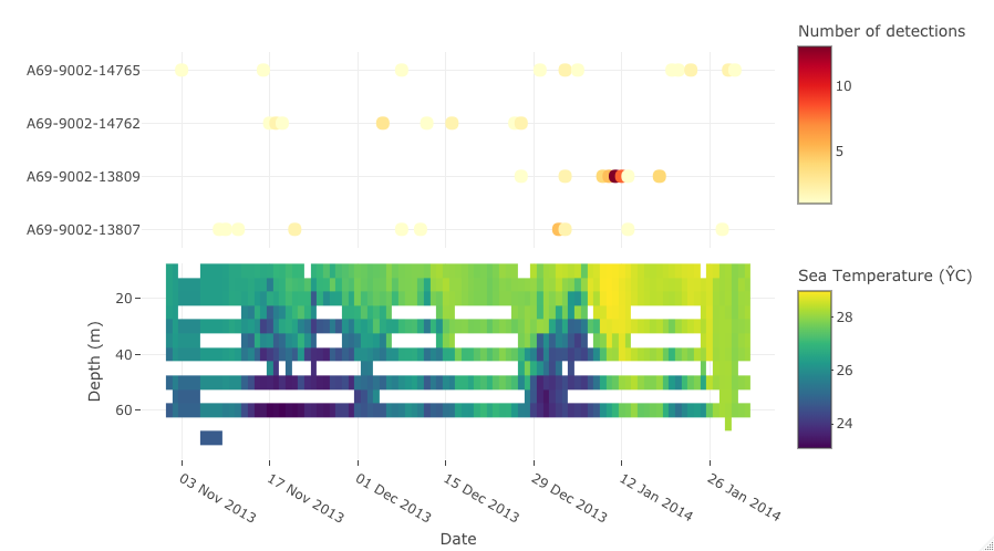

We can also visualise current velocity data with the detections, where moorings have velocity sensors. For example, we can visualise the zonal, North-South (v) velocity (vcur) at the the same mooring, and plot the bull shark detections associated with that mooring.

We need to make sure that the NetCDF file we have stored locally contains the velocity data. To achieve this, we firstly need to download this netCDF file using the mooringDownload() function and then save the file to a different folder location, in this case imos.cache/moor/velocity.

plotDat.l <- mooringDownload(moor_site_codes = "GBRPPS", 
                             fromWeb = TRUE, # Download the netCDF. If already downloaded, set as FALSE
                             sensorType="velocity", # sensor data to download
                             file_loc="imos.cache/moor/velocity", # Location where the netCDF is stored/saved
                             itimeout=240) 
            
# plot the moorings data
plotDT(moorData=plotDat.l$GBRPPS, 
       moorName="GBRPPS",
       dateStart="2013-11-01", 
       dateEnd="2014-02-01", 
       varName = "vcur",
       trackingData=det_dist,
       speciesID="Carcharhinus leucas",
       IDtype="species_scientific_name",
       detStart="2013-11-01",
       detEnd="2014-02-01")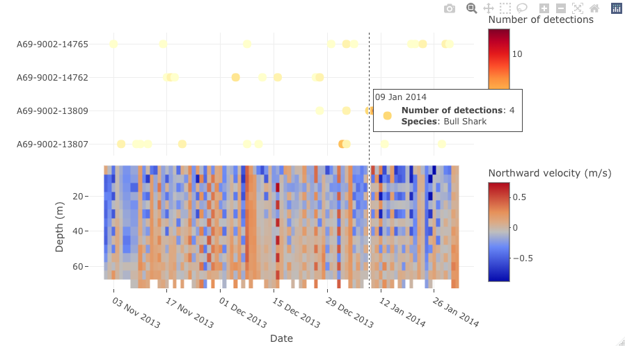

Moorings data extraction

Say we wanted to match each animal tag detection to the nearest mooring sensor value. How would we achieve this?

In this example, we will extract moorings derived water temperature collected from the nearest sensor in the IMOS National Mooring Network to a tag detection at an acoustic receiver.

Sea water temperature, current velocity, or salinity data can be accessed one at a time using the extractMoor() function. There are a few parameters within the function that can help the user identify the variable required, and to manage the downloaded environmental layers:

trackingData: the data frame with the detection data
file_loc: the name of the folder where the NetCDF files for the moorings are stored
sensorType: name of mooring sensor to query. Can be temperature, velocity or salinity.
timeMaxh: optional numeric string containing the maximum time threshold in hours to merge detection and mooring sensor values. The default value is Inf, which allows to run the function without a timeout threshold.
distMaxkm: optional numeric string containing the maximum distance threshold in kilometers to include in output. The default value is Inf, which allows to run the function without distance threshold.
targetDepthm: extracts the nearest sensor to this depth value. The default value is NA, which returns all sensor records at this mooring
scalc: when there are two options for sensors nearest the idepth provided, should the lower (min) or higher (max) depth value be returned? Users can also specify a mean of the available values, or NA to return both sensor values.

By default, each of the environmental sensors positioned on a mooring will be returned for a certain timestamp. For example, if 10 sensors are positioned on a mooring, each hourly timestamp for that mooring witll have 10 sensor readings.

data_with_mooring_sst_all <- extractMoor(trackingData = det_dist,
                                         file_loc="imos.cache/moor/temperature",
                                         sensorType = "temperature",
                                         timeMaxh = Inf,
                                         distMaxkm = Inf)

We can see the extracted environmental variables are appended as new columns to the input dataset as a nested tibble. You can look at the contents of this by using the unnest() function in the tidyr package.

data_with_mooring_sst_all # By default the output is a nested tibble

# Unnest tibble to reveal the first 10 rows of the data
data_with_mooring_sst_all %>% 
  tidyr::unnest(cols = c(data))

If we wanted to extract the sensor positioned at the shallowest depth available on a mooring, we can do so by setting the parameter idepth = 0. Alternatively if there is a preferred depth at which you would like to extract, the function will select the nearest sensor to this value.

You can increase the sensitivity of the extractMoor() function by setting a maximum time threshold (in hours) for the period you are willing to allow between tag detection and mooring timestamps (timeMaxh). You can also add a distance threshold (distMaxkm) for maximum allowed distance (in kilometers) between moorings and receiver station locations.

In this example, we will limit our function so that only detections within 24h and 50km of moorings are allocated with sensor value readings.

As each mooring line has multiple sensors deployed at various depths, we can specify which sensor we want returned by setting a targetDepthm. Here we set this as targetDepthm=0 to return the sensor value that is nearest to the water surface.

# Run the same function again with time and distance thresholds
# and when multiple sensors are available return the shallowest value at that time stamp
data_with_mooring_sst_shallow <- extractMoor(trackingData = det_dist,
                                             file_loc="imos.cache/moor/temperature",
                                             sensorType = "temperature",
                                             timeMaxh = 24,
                                             distMaxkm = 50,
                                             targetDepthm=0, 
                                             scalc="min")

data_with_mooring_sst_shallow

Notice that this new merged dataset data_with_mooring_sst_shallow is now much smaller than the original one data_with_mooring_sst_all? This is because we have extracted only selected a single sensor value for each detection timestamp. We have also dropped those rows from the dataset which not did meet the time and distance thresholds.

Examining the appended environmental data

Now let’s see how the detections of our tagged animals corresponded with variations in sea water temperature. First let’s add the in-situ temperature values to the detection plots grouped by transmitter_id:

summarised_data_id <-
  data_with_mooring_sst_shallow %>% 
  tidyr::unnest(cols = c(data)) %>% 
  mutate(date = as.Date(detection_datetime)) %>% 
  group_by(transmitter_id, date) %>% 
  dplyr::summarise(num_det = n(),
            mean_temperature = mean(moor_sea_temp, na.rm = T))

library(ggplot2)
ggplot(summarised_data_id, aes(x = date, y = transmitter_id, size = num_det, color = mean_temperature)) +
  geom_point() +
  scale_color_viridis_c() +
  labs(subtitle = "In-situ sea water temperature (°C)") +
  theme_bw()

Alternatively we can view the appended detection plots grouped by station_name for only those installations which have mooring sensor data associated with it:

summarised_data_id <-
  data_with_mooring_sst_shallow %>% 
  tidyr::unnest(cols = c(data)) %>% 
  mutate(date = as.Date(detection_datetime)) %>% 
  group_by(installation_name, date) %>% 
  dplyr::summarise(num_det = n(),
            mean_temperature = mean(moor_sea_temp, na.rm = T)) #%>% drop_na(mean_temperature)


ggplot(summarised_data_id, aes(x=date,y=installation_name,
                               size=num_det,color=mean_temperature)) +
  geom_point() +
  scale_color_viridis_c() +
  labs(subtitle = "In-situ sea water temperature (°C)") +
  theme_bw()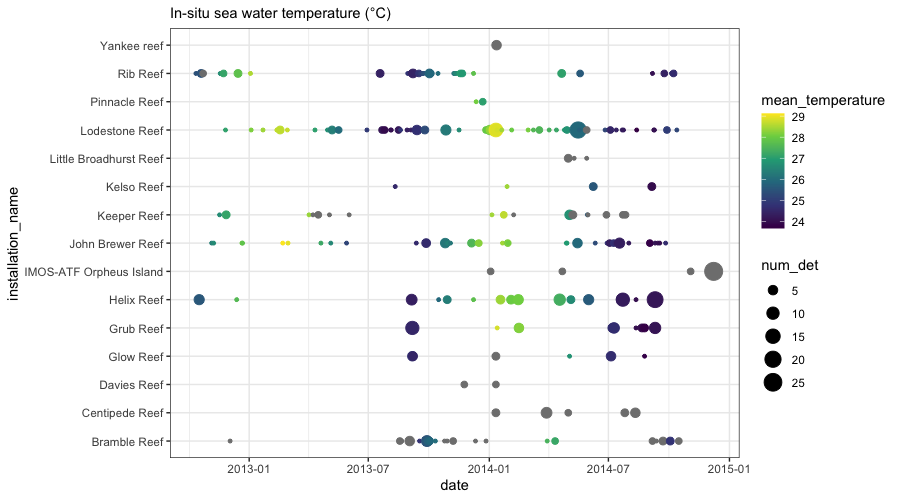

Finally, we can plot the sensor values associated to a detection as a histogram showing the number of detection records associated with each sensor value.

library(hrbrthemes)
# First plot the temperature data
data_with_mooring_sst_shallow %>% 
  tidyr::unnest(cols = c(data)) %>% 
  ggplot(aes(x=moor_sea_temp)) +
  geom_histogram(binwidth=1,fill="#69b3a2",color="#e9ecef",alpha=0.9) +
  facet_wrap(~installation_name,scales="free_y",drop=TRUE) +
  ggtitle("In-situ sea water temperatures when bull sharks present (°C)") +
  #theme_ipsum() +
  theme(
    plot.title = element_text(size=15)
  )

# Next plot the depth data
data_with_mooring_sst_shallow %>% 
  tidyr::unnest(cols = c(data)) %>% 
  drop_na(moor_sea_temp) %>%
  ggplot(aes(x=moor_depth)) +
  geom_histogram(binwidth=5, fill="#69b3a2", color="#e9ecef", alpha=0.9) +
  ggtitle("Depths of sea water temperature readings (m)") +
  theme_ipsum() +
  theme(
    plot.title = element_text(size=15)
  )

Vignette version 0.1.2 (05 Nov 2021)

Integrating in-situ moorings data from the National Mooring Network with QC’d animal detections