extractBlue

This functionality of the remora package allows users to integrate acoustic telemetry data and Bluelink (BRAN) environmental data. Since this is a reanalysis data with 10-km spatial resolution, the user will benefit from a dataset with daily resolution and no gaps, which are common in remotely sensed data due to cloud cover. Again, we advocate for users to first undertake a quality control step using the runQC() function and workflow before further analysis (see vignette('runQC')), however the functionality to append Bluelink (BRAN) environmental data will work on any dataset that has at the minimum spatial coordinates and a timestamp for each detection event. A benefit of using Bluelink (BRAN) data in your analyses of animal movements is that data can be obtained in 3D, ranging from the ocean surface all the way to 4,509 m in depth.

The extractBlue() function can be used to obtain environmental data anywhere in the world.

Example of Bluelink (BRAN) water temperature data at the surface on 1 January 2013 showing its global coverage

Types of environmental data

This function allows users to download and process a range of daily oceanographic variables (between 1993 - present) housed within the Bluelink (BRAN). Information about the Bluelink (BRAN) variables currently avaiable for download using remora can be found using imos_variables(). These datasets can also be manually downloaded with daily, weekly or annual resolutions through the NCI portal.

Variables include current speed at both horizontal (in both x (u) and y (v) directions) and vertical planes (i.e. ocean_w will provide data on current speed in the vertical plane), and other environmental variables at depths ranging between the ocean surface to 4,905 m.

library(remora)

imos_variables()

Variable	Platform	Temporal resolution	Units	Function to use	Description	Source
bathy	Composite raster product		meters	extractEnv()	Australian Bathymetry and Topography Grid. 250 m resolution.	Geosciences Australia
dist_to_land	Raster product		kilometers	extractEnv()	Distance from nearest shoreline (in km). Derived from the high-resolution Open Street Map shoreline product.	This package
rs_sst	Satellite-derived raster product	daily (2002-07-04 - present)	degrees Celcius	extractEnv()	1-day multi-swath multi-sensor (L3S) remotely sensed sea surface temperature (degrees Celcius) at 2 km resolution. Derived from the Group for High Resolution Sea Surface Temperature (GHRSST)	IMOS
rs_sst_interpolated	Raster product	daily (2006-06-12 - present)	degrees Celcius	extractEnv()	1-day interpolated remotely sensed sea surface temperature (degrees Celcius) at 9 km resolution. Derived from the Regional Australian Multi-Sensor Sea surface temperature Analysis (RAMSSA, Beggs et al. 2010) system as part of the BLUElink Ocean Forecasting Australia project	IMOS
rs_chl	Satellite-derived raster product	daily (2002-07-04 - present)	mg.m-3	extractEnv()	Remotely sensed chlorophyll-a concentration (OC3 model). Derived from the MODIS Aqua satellite mission. Multi-spectral measurements are used to infer the concentration of chlorophyll-a, most typically due to phytoplankton, present in the water (mg.m-3).	IMOS
rs_current	Composite raster product	daily (1993-01-01 - present)	ms-1; degrees	extractEnv()	Gridded (adjusted) sea level anomaly (GSLA), surface geostrophic velocity in the east-west (UCUR) and north-south (VCUR) directions for the Australasian region derived from the IMOS Ocean Current project. Two additional variables are calculated: surface current velocity (ms-1) and bearing (degrees).	IMOS
rs_salinity	Satellite-derived raster product	weekly (2011-08-25 - 2015-06-07)	psu	extractEnv()	7-day composite remotely sensed salinity. Derived from the NASA Aquarius satellite mission (psu).	IMOS
rs_turbidity	Satellite-derived raster product	daily (2002-07-04 - present)	m-1	extractEnv()	Diffuse attenuation coefficient at 490 nm (K490) indicates the turbidity of the water column (m-1). The value of K490 represents the rate which light at 490 nm is attenuated with depth. For example a K490 of 0.1/meter means that light intensity will be reduced one natural log within 10 meters of water. Thus, for a K490 of 0.1, one attenuation length is 10 meters. Higher K490 value means smaller attenuation depth, and lower clarity of ocean water.	IMOS
rs_npp	Satellite-derived raster product	daily (2002-07-04 - present)	mgC.m_2.day-1	extractEnv()	Net primary productivity (OC3 model and Eppley-VGPM algorithm). Modelled product used to compute an estimate of the Net Primary Productivity (NPP). The model used is based on the standard vertically generalised production model (VGPM). The VGPM is a “chlorophyll-based” model that estimates net primary production from chlorophyll using a temperature-dependent description of chlorophyll-specific photosynthetic efficiency. For the VGPM, net primary production is a function of chlorophyll, available light, and the photosynthetic efficiency. The only difference between the Standard VGPM and the Eppley-VGPM is the temperature-dependent description of photosynthetic efficiencies, with the Eppley approach using an exponential function to account for variation in photosynthetic efficiencies due to photoacclimation.	IMOS
moor_sea_temp	Fixed sub-surface moorings	hourly	degrees Celcius	extractMoor()	Depth-integrated in-situ, hourly time-series measurements of sea temperature (degrees Celcius) at fixed mooring locations	IMOS
moor_psal	Fixed sub-surface moorings	hourly	psu	extractMoor()	Depth-integrated in-situ, hourly time-series measurements of salinity (psu) at fixed mooring locations	IMOS
moor_ucur	Fixed sub-surface moorings	hourly	ms-1	extractMoor()	Depth-integrated in-situ, hourly time-series measurements of subsurface geostrophic current velocity in the east-west direction (ms-1) at fixed mooring locations	IMOS
moor_vcur	Fixed sub-surface moorings	hourly	ms-1	extractMoor()	Depth-integrated in-situ, hourly time-series measurements of subsurface geostrophic current velocity in the north-south direction (ms-1) at fixed mooring locations	IMOS
ocean_temp	3D Raster product	daily (1993-01-01 - present)	degrees Celcius	extractBlue()	Water temperature at specified depth from the surface to 4,509-m depth	Bluelink (CSIRO)
ocean_salt	3D Raster product	daily (1993-01-01 - present)	psu	extractBlue()	Water salinity at specified depth from the surface to 4,509-m depth	Bluelink (CSIRO)
ocean_u	3D Raster product	daily (1993-01-01 - present)	ms-1	extractBlue()	Current horizontal speed component in the x direction at specified depth from the surface to 4,509-m depth	Bluelink (CSIRO)
ocean_v	3D Raster product	daily (1993-01-01 - present)	ms-1	extractBlue()	Current horizontal speed component in the y direction at specified depth from the surface to 4,509-m depth	Bluelink (CSIRO)
ocean_w	3D Raster product	daily (1993-01-01 - present)	ms-1	extractBlue()	Current vertical speed component at specified depth from the surface to 4,509-m depth	Bluelink (CSIRO)
ocean_eta_t	3D Raster product	daily (1993-01-01 - present)	meters	extractBlue()	Sea surface height at the water surface	Bluelink (CSIRO)
ocean_mld	3D Raster product	daily (1993-01-01 - present)	meters	extractBlue()	Mixed layer depth in relation to the water surface	Bluelink (CSIRO)
air_wind	Raster product	daily (1993-01-01 - present)	ms-1; degrees clockwise	extractBlue()	Returns both wind speed (ms-1) and direction (° clockwise) as two separate columns	Bluelink (CSIRO)

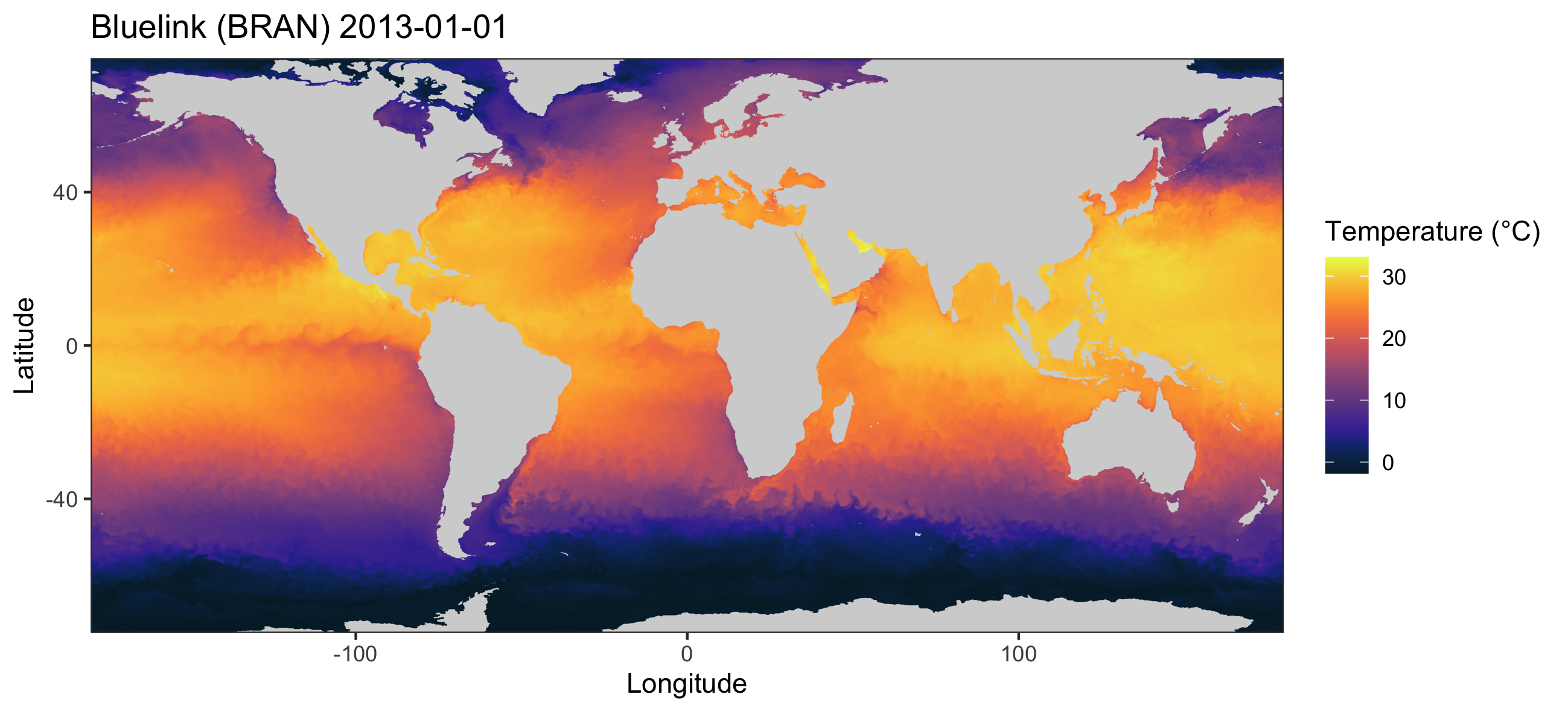
In this vignette we will explore some examples for accessing and integrating Bluelink (BRAN) data, both at depth and at the water surface.

Usage of the `extractBlue()` function

Load example dataset

The primary function to extract and append Bluelink (BRAN) data to telemetry data is the extractBlue() function. Lets start with a dataset that has undergone quality control (see vignette('runQC')).

library(tidyverse)
library(raster)
library(ggspatial)

## Example dataset that has undergone quality control using the `runQC()` function
data("TownsvilleReefQC")

## Only retain detections flagged as 'valid' and 'likely valid' (Detection_QC 1 and 2)
qc_data <- 
   TownsvilleReefQC %>% 
   unnest(cols = c(QC)) %>% 
   ungroup() %>% 
   filter(Detection_QC %in% c(1,2)) %>%
   filter(filename == unique(filename)[1]) %>%
   slice(1:20)

For an overview on the spatial and temporal patterns in this example dataset please see the extractEnv() vignette.

Bluelink (BRAN) environmental data extraction

In this example, we will extract two variables; water temperature at depth (30 m) and surface 3D current speeds.

Each variable will need to be accessed one at a time using the extractBlue() function. There are a few parameters within the function that can help the user identify the variable required, and to manage the downloaded environmental layers:

df: the data frame with the detection data
X: the name of the column with longitude for each detection
Y: the name of the column with latitude for each detection
datetime: the name of the column with the date-timestamp for each detection
env_var: the name of the environmental variable to download and append (see imos_variables() for available variables and variable names)
extract_depth: since the Bluelink (BRAN) data is 3D, the user can define a specific depth of interest and the function will obtain the environmental data at the nearest layer available. By default, data is obtained at the water surface (extract_depth = 0).
cache_layers: should the extracted and processed environmental data layers be cached within the working directory? If so, spatial layers will be cached in a folder (folder_name) within your working directory, and named after the environmental variable of interest. Since the raw files downloaded have a global resolution, for computational purposes these exported files will encompass only your study area
full_timeperiod: should environmental variables extracted for each day across full monitoring period? If set to TRUE it can be time and memory consuming for long projects

Running the function with `full_timeperiod = TRUE`

If this option is selected the extractBlue function will standardize the acoustic dataset for further analyses. This option can be very time consuming, depending on the duration of the study and number of acoustic stations included. During standardization, information at individual level will be lost, and the exported dataset will be sorted by acoustic station (station_name column) and date (detection_datetime column converted to Date format). A new column Detection will be included, and will comprise 1 (days with detections) and 0 (days without detections) values:

## Obtain standardized data with water temperatures at the surface:
standdata_with_sst <- 
    extractBlue(df = qc_data,
                X = "receiver_deployment_longitude", 
                Y = "receiver_deployment_latitude", 
                station_name = "station_name",
                datetime = "detection_datetime", 
                env_var = "ocean_temp",
                extract_depth = 0,
                cache_layers = FALSE,
                export_step = FALSE,
                verbose = TRUE,
                full_timeperiod = TRUE)

If we have a look at this dataset it will look like this:

date	station_name	lon	lat	ocean_temp_0	Detection
2013-08-10	Kelso 2	146.991	-18.417	23.5647	1
2013-08-11	Kelso 2	146.991	-18.417	23.5492	0
2013-08-12	Kelso 2	146.991	-18.417	24.1562	0
2013-08-13	Kelso 2	146.991	-18.417	24.1873	0
2013-08-14	Kelso 2	146.991	-18.417	24.1951	0
2013-08-15	Kelso 2	146.991	-18.417	24.3274	0

Which means that, on (2013-08-10) detections were recorded at the Kelso 2 station (Detection = 1), but not on the other days in the example (Detection = 0), but temperature data at the surface (ocean_temp_0) was extracted for all days.

Gap filling functionality

While cloud cover is not a limitation to obtain Bluelink (BRAN) environmental data at oceanic regions, those locations in very close proximity to the coast might return NA values. In these cases, you can use the fill_gaps and buffer arguments (similar to their uses in extractEnv()) to fill the rows with missing information. By default, fill_gaps is set to FALSE and buffer is set to 10-km (i.e. the same resolution as the raw environmental data).

These two arguments can be particularly usefull if the user wants to extract environmental data at depths deeper than the deployment locations of the acoustic receivers.

For example, if we want to extract water temperature data at 40-m depth without the gap filling function, we would get the following output:

 data1_with_temp40 <- 
    extractBlue(df = qc_data,
                X = "receiver_deployment_longitude", 
                Y = "receiver_deployment_latitude", 
                datetime = "detection_datetime", 
                env_var = "ocean_temp",
                extract_depth = 40,
                cache_layers = FALSE,
                verbose = TRUE,
                fill_gaps = FALSE)

summary(data1_with_temp40$ocean_temp_40)

ocean_temp_40
Min.   :23.44
1st Qu.:23.53
Median :23.60
Mean   :23.75
3rd Qu.:23.83
Max.   :24.70
NA's   :12

Which means that, 12 stations (out of 20) were located in depths shallower than 40 m. Therefore, we can use the gap filling function to obtain data at the nearest 40-m available pixels by using a 25-km buffer:

 data2_with_temp40 <- 
    extractBlue(df = qc_data,
                X = "receiver_deployment_longitude", 
                Y = "receiver_deployment_latitude", 
                datetime = "detection_datetime", 
                env_var = "ocean_temp",
                extract_depth = 40,
                cache_layers = FALSE,
                verbose = TRUE,
                fill_gaps = TRUE,
                buffer = 25000) # use a 25-km buffer

summary(data2_with_temp40$ocean_temp_40)

ocean_temp_40
Min.   :23.44
1st Qu.:23.77
Median :23.32
Mean   :23.12
3rd Qu.:23.37
Max.   :24.70

Water temperature at depth (30 m)

We are going to use the function to compare the water temperatures in the study area between the surface and the 30-m depths. Let’s download and process the Bluelink (BRAN) data at the two depths of interest:

## Obtain water temperature data at the surface
data_with_sst1 <- 
  extractBlue(df = qc_data,
             X = "receiver_deployment_longitude", 
             Y = "receiver_deployment_latitude", 
             datetime = "detection_datetime", 
             cache_layers = FALSE,
             env_var = "ocean_temp",
             extract_depth = 0) # surface

## Obtain water temperature data at the 30-m depths
data_with_sst2 <- 
  extractBlue(df = qc_data,
             X = "receiver_deployment_longitude", 
             Y = "receiver_deployment_latitude", 
             datetime = "detection_datetime", 
             cache_layers = FALSE,
             env_var = "ocean_temp",
             extract_depth = 30) # 30-m depths

Now let’s see how the two variables look in relation to each other:

data_plot <- data.frame(Station = data_with_sst1$station_name,
  Date = data_with_sst1$detection_datetime,
  Variable = c(rep("Surface", nrow(data_with_sst1)), rep("Depth", nrow(data_with_sst1))),
  Temperature = c(data_with_sst1$ocean_temp_0, data_with_sst2$ocean_temp_30))
data_plot$Variable <- factor(data_plot$Variable, levels = c("Surface", "Depth"))

ggplot() + theme_bw() +
  geom_boxplot(data = data_plot, aes(x = Station, y = Temperature, colour = Variable)) +
  labs(y = "Temperature (°C)", colour = "")

Surface 3D current speeds

We can also use the extractBlue() function to obtain 3D current data along our study region. In this example, we are going to download horizontal (u and v components) and vertical current data, and save the processed Bluelink (BRAN) files for further investigation. First, let’s download the data:

# download u-current data (horizontal x-direction)
data_cur <- 
    extractBlue(df = qc_data,
                X = "receiver_deployment_longitude", 
                Y = "receiver_deployment_latitude", 
                datetime = "detection_datetime", 
                env_var = "ocean_u",
                extract_depth = 0,
                cache_layers = TRUE,
                verbose = TRUE)

# download v-current data (horizontal y-direction)
data_cur <- 
    extractBlue(df = data_cur,
                X = "receiver_deployment_longitude", 
                Y = "receiver_deployment_latitude", 
                datetime = "detection_datetime", 
                env_var = "ocean_v",
                extract_depth = 0,
                cache_layers = TRUE,
                verbose = TRUE)

# download w-current data (vertical direction)
data_cur <- 
    extractBlue(df = data_cur,
                X = "receiver_deployment_longitude", 
                Y = "receiver_deployment_latitude", 
                datetime = "detection_datetime", 
                env_var = "ocean_w",
                extract_depth = 0,
                cache_layers = TRUE,
                verbose = TRUE)

As we set cache_layers to TRUE, the downloaded and processed files will be cached in the folder_name folder within the working directory, in a folder called cached. We can then load these processed files and plot them, to look at the trends in current speed within the study area:

# Load processed netCDF files:
nc.u <- brick("Bluelink/Bluelink_ocean_u_0.nc")
nc.v <- brick("Bluelink/Bluelink_ocean_v_0.nc")
nc.w <- brick("Bluelink/Bluelink_ocean_w_0.nc")

# Convert to data frame for plotting (first day of data)
df.u <- as.data.frame(nc.u[[1]], xy = TRUE)
df.v <- as.data.frame(nc.v[[1]], xy = TRUE)
df.w <- as.data.frame(nc.w[[1]], xy = TRUE)

# Plot variables
library(cmocean) 
library(patchwork)
library(ozmaps)
oz_states <- ozmap_states # load Australia shapefile

plot1 <- ggplot() + theme_bw() +
  geom_raster(data = df.u, aes(x = x, y = y, fill = X1)) +
  scale_fill_gradientn(colours = cmocean("balance")(100), na.value = NA, limits = c(-0.37, 0.37)) +
  geom_sf(data = oz_states, fill = "lightgray", colour = "darkgray", lwd = 0.2, alpha = 0.5) +
  coord_sf(xlim = c(145.7, 148.1), ylim = c(-19.7, -17.3), expand = FALSE) + 
  geom_point(data = qc_data, 
    aes(x = receiver_deployment_longitude, y = receiver_deployment_latitude)) + 
  labs(x = "", y = "", title = "u-current", fill = "Speed (m/s)") +
  scale_x_continuous(breaks = seq(146, 148, 1)) +
  theme(legend.position = "bottom")

plot2 <- ggplot() + theme_bw() +
  geom_raster(data = df.v, aes(x = x, y = y, fill = X1)) +
  scale_fill_gradientn(colours = cmocean("balance")(100), na.value = NA, limits = c(-0.37, 0.37)) +
  geom_sf(data = oz_states, fill = "lightgray", colour = "darkgray", lwd = 0.2, alpha = 0.5) +
  coord_sf(xlim = c(145.7, 148.1), ylim = c(-19.7, -17.3), expand = FALSE) + 
  geom_point(data = qc_data, 
    aes(x = receiver_deployment_longitude, y = receiver_deployment_latitude)) + 
  labs(x = "", y = "", title = "v-current", fill = "Speed (m/s)") +
  scale_x_continuous(breaks = seq(146, 148, 1)) +
  theme(legend.position = "bottom")

plot3 <- ggplot() + theme_bw() +
  geom_raster(data = df.w, aes(x = x, y = y, fill = X1)) +
  scale_fill_gradientn(colours = cmocean("balance")(100), na.value = NA, limits = c(-4e-05, 4e-05),
    breaks = c(-4e-05, 0, 4e-05)) +
  geom_sf(data = oz_states, fill = "lightgray", colour = "darkgray", lwd = 0.2, alpha = 0.5) +
  coord_sf(xlim = c(145.7, 148.1), ylim = c(-19.7, -17.3), expand = FALSE) + 
  geom_point(data = qc_data, 
    aes(x = receiver_deployment_longitude, y = receiver_deployment_latitude)) + 
  labs(x = "", y = "", title = "w-current", fill = "Speed (m/s)") +
  scale_x_continuous(breaks = seq(146, 148, 1)) +
  theme(legend.position = "bottom")

plot1 + plot2 + plot3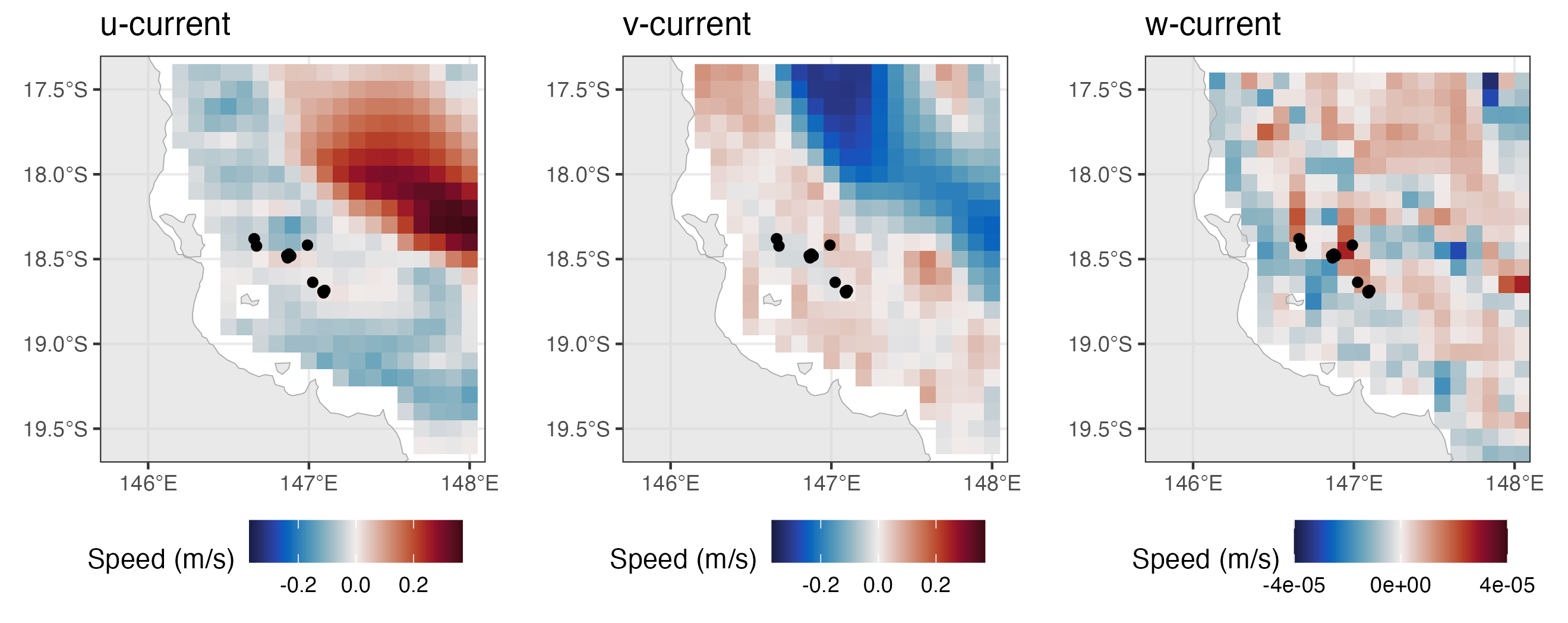

Vignette version 0.0.1 (26 Jun 2023)

Integrating Bluelink (BRAN) environmental data with animal locations