extractEnv
Integrating remotely sensed environmental data with QC’d animal detections
Source:vignettes/extractEnv.Rmd
extractEnv.RmdAnother key functionality of the remora package allows
users to integrate acoustic telemetry data and environmental and habitat
information. This package allows the user to match a range of
environmental variables to each detection. Associating environmental
data to detections provides a means to analyse environmental or habitat
drivers of occurrence, presence and movement of animal monitored using
acoustic telemetry. We advocate for users to first undertake a quality
control step using the runQC() function and workflow before
further analysis (see vignette('runQC')), however the
functionality to append environmental data will work on any dataset that
has at the minimum spatial coordinates and a timestamp for each
detection event.
Currently, the focus of this package is to integrate animal telemetry data and environmental data collated by Australia’s Integrated Marine Observing System. Therefore, the geographical scope of available datasets is currently restricted to the Australiasia region. As this package develops, more sources of environmental data will be added to enable users to access more datasets across Australia and globally.
Types of environmental data
This package allows users to access a range of ocean observing datasets that have undergone a quality control process and housed within the Integrated Marine Observing System. These datasets can also be explored through the Australian Ocean Data Network portal. There are primarily two types of environmental data that users can currently access:
1. Remotely-sensed or gridded environmental data
2. In situ sub-surface environmental data from moorings at fixed locations
The imos_variables() function will help the user
identify currently available environmental layers that can be accessed
and associated. Variables include spatial layers including
bathy and dist_to_land, which provide distance
measures of bathymetry (in meters) and proximity to land (in
kilometers). Variable names that start with rs_ are
remotely-sensed or gridded environmental layers, and variables starting
with moor_ include in situ sub-surface mooring
environmental layers.
| Variable | Platform | Temporal resolution | Units | Function to use | Description | Source |
|---|---|---|---|---|---|---|
| bathy | Composite raster product |
|
meters | extractEnv() | Australian Bathymetry and Topography Grid. 250 m resolution. | Geosciences Australia |
| dist_to_land | Raster product |
|
kilometers | extractEnv() | Distance from nearest shoreline (in km). Derived from the high-resolution Open Street Map shoreline product. | This package |
| rs_sst | Satellite-derived raster product | daily (2002-07-04 - present) | degrees Celcius | extractEnv() | 1-day multi-swath multi-sensor (L3S) remotely sensed sea surface temperature (degrees Celcius) at 2 km resolution. Derived from the Group for High Resolution Sea Surface Temperature (GHRSST) | IMOS |
| rs_sst_interpolated | Raster product | daily (2006-06-12 - present) | degrees Celcius | extractEnv() | 1-day interpolated remotely sensed sea surface temperature (degrees Celcius) at 9 km resolution. Derived from the Regional Australian Multi-Sensor Sea surface temperature Analysis (RAMSSA, Beggs et al. 2010) system as part of the BLUElink Ocean Forecasting Australia project | IMOS |
| rs_chl | Satellite-derived raster product | daily (2002-07-04 - present) | mg.m-3 | extractEnv() | Remotely sensed chlorophyll-a concentration (OC3 model). Derived from the MODIS Aqua satellite mission. Multi-spectral measurements are used to infer the concentration of chlorophyll-a, most typically due to phytoplankton, present in the water (mg.m-3). | IMOS |
| rs_current | Composite raster product | daily (1993-01-01 - present) | ms-1; degrees | extractEnv() | Gridded (adjusted) sea level anomaly (GSLA), surface geostrophic velocity in the east-west (UCUR) and north-south (VCUR) directions for the Australasian region derived from the IMOS Ocean Current project. Two additional variables are calculated: surface current velocity (ms-1) and bearing (degrees). | IMOS |
| rs_salinity | Satellite-derived raster product | weekly (2011-08-25 - 2015-06-07) | psu | extractEnv() | 7-day composite remotely sensed salinity. Derived from the NASA Aquarius satellite mission (psu). | IMOS |
| rs_turbidity | Satellite-derived raster product | daily (2002-07-04 - present) | m-1 | extractEnv() | Diffuse attenuation coefficient at 490 nm (K490) indicates the turbidity of the water column (m-1). The value of K490 represents the rate which light at 490 nm is attenuated with depth. For example a K490 of 0.1/meter means that light intensity will be reduced one natural log within 10 meters of water. Thus, for a K490 of 0.1, one attenuation length is 10 meters. Higher K490 value means smaller attenuation depth, and lower clarity of ocean water. | IMOS |
| rs_npp | Satellite-derived raster product | daily (2002-07-04 - present) | mgC.m_2.day-1 | extractEnv() | Net primary productivity (OC3 model and Eppley-VGPM algorithm). Modelled product used to compute an estimate of the Net Primary Productivity (NPP). The model used is based on the standard vertically generalised production model (VGPM). The VGPM is a “chlorophyll-based” model that estimates net primary production from chlorophyll using a temperature-dependent description of chlorophyll-specific photosynthetic efficiency. For the VGPM, net primary production is a function of chlorophyll, available light, and the photosynthetic efficiency. The only difference between the Standard VGPM and the Eppley-VGPM is the temperature-dependent description of photosynthetic efficiencies, with the Eppley approach using an exponential function to account for variation in photosynthetic efficiencies due to photoacclimation. | IMOS |
| moor_sea_temp | Fixed sub-surface moorings | hourly | degrees Celcius | extractMoor() | Depth-integrated in-situ, hourly time-series measurements of sea temperature (degrees Celcius) at fixed mooring locations | IMOS |
| moor_psal | Fixed sub-surface moorings | hourly | psu | extractMoor() | Depth-integrated in-situ, hourly time-series measurements of salinity (psu) at fixed mooring locations | IMOS |
| moor_ucur | Fixed sub-surface moorings | hourly | ms-1 | extractMoor() | Depth-integrated in-situ, hourly time-series measurements of subsurface geostrophic current velocity in the east-west direction (ms-1) at fixed mooring locations | IMOS |
| moor_vcur | Fixed sub-surface moorings | hourly | ms-1 | extractMoor() | Depth-integrated in-situ, hourly time-series measurements of subsurface geostrophic current velocity in the north-south direction (ms-1) at fixed mooring locations | IMOS |
| BRAN_temp | 3D Raster product | daily (1993-01-01 - 2025-12-31) | degrees Celcius | extractBlue() | Water temperature at specified depth from the surface to 4,509-m depth | Bluelink (CSIRO) |
| BRAN_salt | 3D Raster product | daily (1993-01-01 - 2025-12-31) | psu | extractBlue() | Water salinity at specified depth from the surface to 4,509-m depth | Bluelink (CSIRO) |
| BRAN_cur | 3D Raster product | daily (1993-01-01 - 2025-12-31) | ms-1; degrees clockwise | extractBlue() | Geostrophic velocity in the east-west (UCUR) and north-south (VCUR) directions from the surface to 4,509-m depth. Two additional variables are calculated: current velocity (ms-1) and bearing (degrees). | Bluelink (CSIRO) |
| BRAN_wcur | Raster product | daily (1993-01-01 - 2025-12-31) | ms-1 | extractBlue() | Vertical current speed in the water column is calculated (negative = downwards; positive = upwards) using the layers available between the surface to 200-m depths. | Bluelink (CSIRO) |
| BRAN_ssh | Raster product | daily (1993-01-01 - 2025-12-31) | meters | extractBlue() | Sea surface height at the water surface | Bluelink (CSIRO) |
| BRAN_mld | Raster product | daily (1993-01-01 - 2025-12-31) | meters | extractBlue() | Mixed layer depth in relation to the water surface | Bluelink (CSIRO) |
| BRAN_wind | Raster product | daily (1993-01-01 - 2025-12-31) | ms-1; degrees clockwise | extractBlue() | Wind forcing at the water surface in the east-west (uwind) and north-south (vwind) directions. Two additional variables are calculated: wind velocity (ms-1) and bearing (degrees). | Bluelink (CSIRO) |
In this vignette we will explore accessing and integrating gridded
data. A suite of additional functions can be used to access and extract
in situ sub-surface data from moorings (see
vignette('extractMoor')).
Usage of the extractEnv() function
Load example dataset
The primary function to extract and append remote sensing data to
acoustic detection data is the extractEnv() function. Lets
start with a dataset that has undergone quality control (see
vignette('runQC')).
library(tidyverse)
library(raster)
library(ggspatial)

## Example dataset that has undergone quality control using the `runQC()` function
data("TownsvilleReefQC")

## Only retain detections flagged as 'valid' and 'likely valid' (Detection_QC 1 and 2)
qc_data <-
  TownsvilleReefQC %>%
  tidyr::unnest(cols = QC) %>%
  dplyr::ungroup() %>%
  filter(Detection_QC %in% c(1,2))
Lets have a quick look at the spatial patterns in detection data:
qc_data %>%
  group_by(transmitter_id, station_name, installation_name, receiver_deployment_longitude, receiver_deployment_latitude) %>%
  summarise(num_det = n()) %>%
  ggplot() +
  annotation_map_tile('cartolight') +
  geom_spatial_point(aes(x = receiver_deployment_longitude, y = receiver_deployment_latitude,
                         size = num_det, color = installation_name), crs = 4326) +
  facet_wrap(~transmitter_id, ncol = 2) +
  labs(x = "Longitude", y = "Latitude", color = "Installation Name" , size = "Number of\nDetections") +
  theme_bw()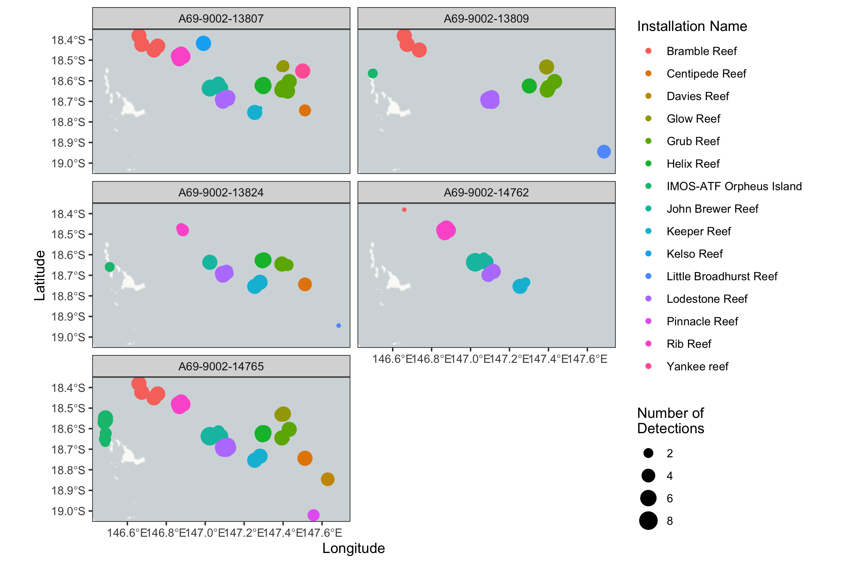
We can also have a look at the temporal pattern in detections:
qc_data %>%
  mutate(date = as.Date(detection_datetime)) %>%
  group_by(transmitter_id, date, installation_name) %>%
  summarise(num_det = n()) %>%
  ggplot(aes(x = date, y = transmitter_id, color = installation_name, size = num_det)) +
  labs(x = "Date", y = NULL, color = "Installation Name", size = "Number of\nDetections") +
  geom_point() +
  theme_bw()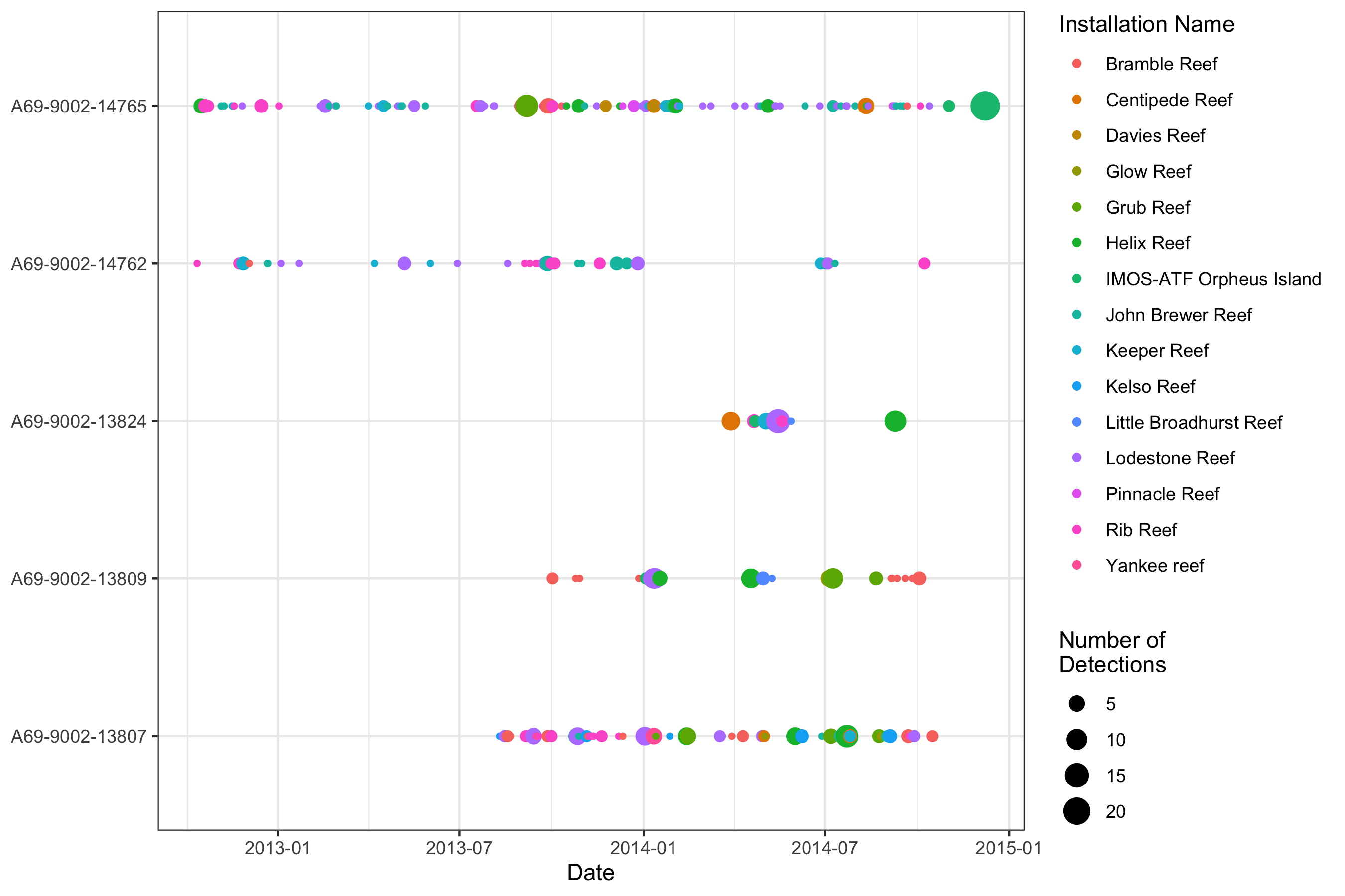
Environmental data extraction
In this example, we will extract two variables; Interpolated sea surface temperature and modeled ocean surface currents.
Each variable will need to be accessed one at a time using the
extractEnv() function. There are a few parameters within
the function that can help the user identify the variable required, and
to manage the downloaded environmental layers:
- df: the data frame with the detection data
- X: the name of the column with longitude for each detection
- Y: the name of the column with latitude for each detection
- datetime: the name of the column with the date-timestamp for each detection
-
env_var: the name of the environmental variable to
download and append (see
imos_variables()for available variables and variable names) -
cache_layers: should the extracted environmental
data layers be cached within the working directory? If so, spatial
layers will be cached within a folder called
imos.cachewithin your working directory. - crop_layers: should the extracted environmental data be cropped to within the study site? reduces the file size of downloaded files
-
full_timeperiod: should environmental variables
extracted for each day across full monitoring period, if set to
TRUEit can be time and memory consuming for long projects -
folder_name: name of folder within
imos.cachewhere downloaded rasters should be saved. If none provided automatic folder names generated based on study extent - .parallel: should the function be run in parallel? speeds up environmental extraction for large datasets
Gap filling functionality
Remote sensed environmental data within coastal areas (where acoustic arrays are often deployed) are often unreliable due to shallow habitats and close proximity to turbid nearshore waters. The quality control process for Ocean colour variables within the IMOS dataset often remove pixels in close proximity to coastlines due to the low quality of environmental variables in these regions. Here is an example where coastal remote sensing data may not match up with positions of deployed acoustic arrays.

In these cases, a simple extraction will result in NAs
where no overlap occurs (e.g., black points in the figure above). To
maximise the understanding of environmental variables in the region of
coastal arrays, extractEnv() provides the functionality to
fill gaps in the extraction data using the fill_gaps
parameter. If fill_gaps = TRUE, the function will extract
the median variable values within a buffer around points that do not
overlap data pixels (broken buffers around black points in the figure
above). The radius of the buffer around the points that do not overlap
data can be user defined (in meters) using the additional
buffer parameter. If no buffer value is
provided by the user, the function will automatically choose a buffer
radius based on the resolution of environmental layer [5 km for
rs_sst, rs_chl, rs_npp,
rs_turbidity; 15 km for rs_sst_interpolated;
20 km for rs_current and rs_salinity].
Interpolated sea surface temperature
data_with_sst <-
  extractEnv(df = qc_data,
             X = "receiver_deployment_longitude",
             Y = "receiver_deployment_latitude",
             datetime = "detection_datetime",
             env_var = "rs_sst_interpolated",  ## Currently only a single variable can be called at a time
             cache_layers = TRUE,
             crop_layers = TRUE,
             fill_gaps = TRUE,
             full_timeperiod = FALSE,
             folder_name = "test",
             .parallel = TRUE)
Modeled ocean surface currents
We can now also append current data to this dataset:
data_with_sst_and_current <-
  data_with_sst %>%
  extractEnv(X = "receiver_deployment_longitude",
             Y = "receiver_deployment_latitude",
             datetime = "detection_datetime",
             env_var = "rs_current",
             cache_layers = TRUE,
             crop_layers = TRUE,
             fill_gaps = TRUE,
             full_timeperiod = FALSE,
             folder_name = "test",
             .parallel = TRUE)
As we set cache_layers to TRUE, the
downloaded layers will be cached within the imos.cache
folder within the working directory. Each time the function is called,
downloaded layers are cached into this folder. We have also set the
function to save the raster layers as the default .grd format within a
subfolder called test.
When downloading current data, three variables are downloaded:
Gridded Sea Level Anomaly (rs_gsla), surface geostrophic
velocity in the north-south direction (rs_vcur) and the
east-west direction (rs_ucur). These variables are used to
calculate current velocity and bearing and appended to detections
Examining the appended environmental data
We can now see the extracted environmental variables are appended as new columns to the input dataset
data_with_sst_and_current## # A tibble: 597 × 61
## filename transmitter_id tag_id transmitter_deployme…¹ tagging_project_name
## <chr> <chr> <int> <int> <chr>
## 1 A69-9002-1… A69-9002-13807 6.99e7 69918684 Townsville Reefs
## 2 A69-9002-1… A69-9002-13807 6.99e7 69918684 Townsville Reefs
## 3 A69-9002-1… A69-9002-13807 6.99e7 69918684 Townsville Reefs
## 4 A69-9002-1… A69-9002-13807 6.99e7 69918684 Townsville Reefs
## 5 A69-9002-1… A69-9002-13807 6.99e7 69918684 Townsville Reefs
## 6 A69-9002-1… A69-9002-13807 6.99e7 69918684 Townsville Reefs
## 7 A69-9002-1… A69-9002-13807 6.99e7 69918684 Townsville Reefs
## 8 A69-9002-1… A69-9002-13807 6.99e7 69918684 Townsville Reefs
## 9 A69-9002-1… A69-9002-13807 6.99e7 69918684 Townsville Reefs
## 10 A69-9002-1… A69-9002-13807 6.99e7 69918684 Townsville Reefs
## # ℹ 587 more rows
## # ℹ abbreviated name: ¹transmitter_deployment_id
## # ℹ 56 more variables: species_common_name <chr>,
## # species_scientific_name <chr>, CAAB_species_id <int>,
## # WORMS_species_aphia_id <int>, animal_sex <chr>, detection_datetime <dttm>,
## # receiver_deployment_longitude <dbl>, receiver_deployment_latitude <dbl>,
## # receiver_project_name <chr>, installation_name <chr>, station_name <chr>, …We can also now add the variables to the detection plots:
summarised_data <-
  data_with_sst_and_current %>%
  mutate(date = as.Date(detection_datetime)) %>%
  group_by(transmitter_id, date) %>%
  summarise(num_det = n(),
            mean_sst = mean(rs_sst_interpolated, na.rm = T),
            mean_current_velocity = mean(rs_current_velocity, na.rm = T),
            mean_current_bearing = mean(rs_current_bearing, na.rm = T))

ggplot(summarised_data, aes(x = date, y = transmitter_id, size = num_det, color = mean_sst)) +
  geom_point() +
  scale_color_viridis_c() +
  labs(subtitle = "Interpolated sea surface temperature", x = "Date",
       y = NULL, color = "SST (˚C)", size = "Number of\nDetections") +
  theme_bw()
ggplot(summarised_data) +
  geom_point(aes(x = date, y = transmitter_id, color = mean_current_velocity,
                 size = num_det)) +
  geom_spoke(aes(x = date, y = transmitter_id, angle = mean_current_bearing, radius = mean_current_velocity),
             arrow = arrow(length = unit(0.05, 'inches')), color = "grey", lwd = 0.1) +
  labs(subtitle = "Direction and velocity of modeled surface currents", x = "Date",
       y = NULL, color = "Current\nVelocity (ms-1)", size = "Number of\nDetections") +
  scale_color_viridis_c(option = "B") +
  theme_bw()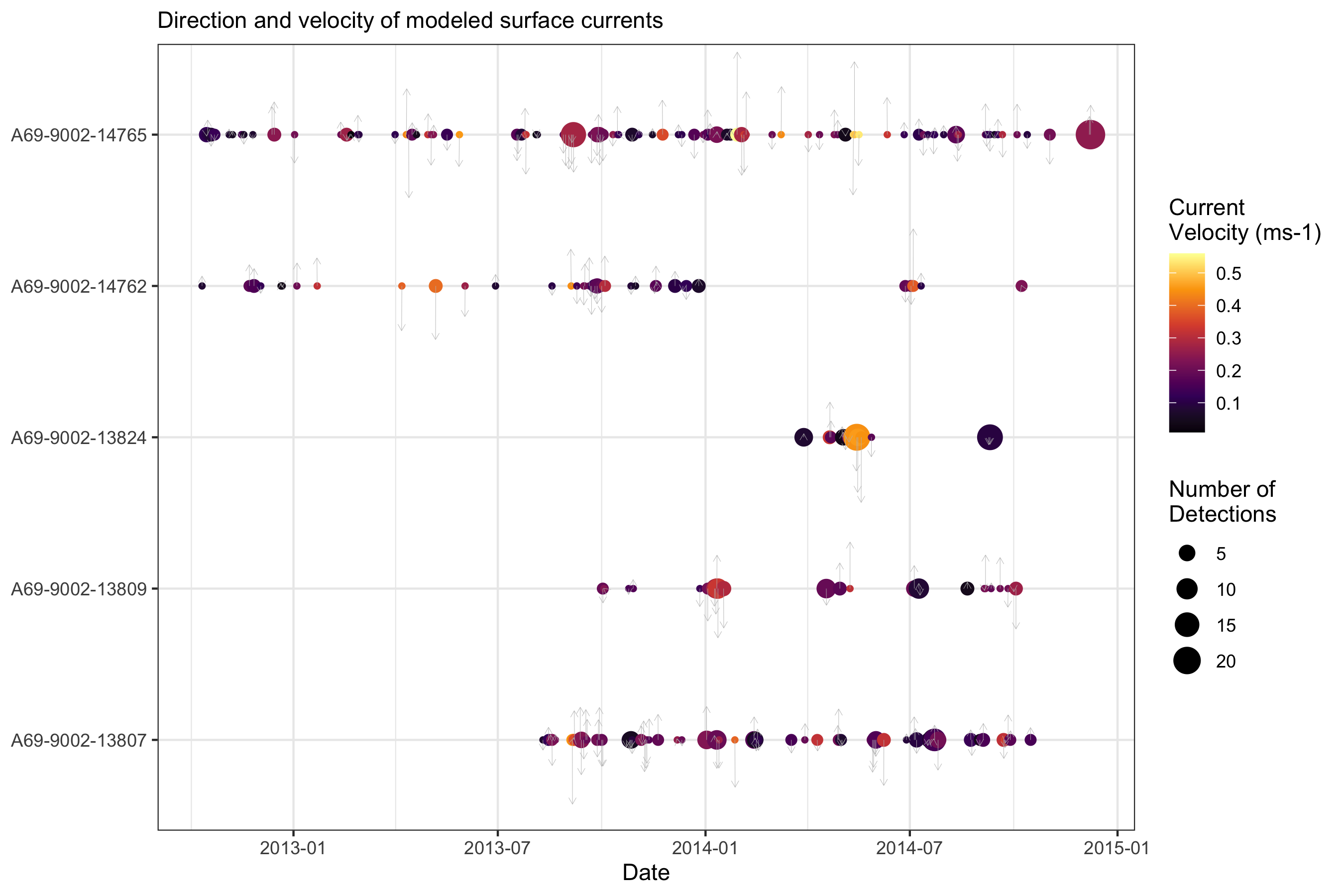
If the environmental layers were cached, we can also look at how the variables altered spatially:
## Detection data summary
det_summary <-
  qc_data %>%
  group_by(station_name, lon = receiver_deployment_longitude, lat = receiver_deployment_latitude) %>%
  summarise()

## Sea surface temperature
sst_raster <- stack("imos.cache/rs variables/test/rs_sst_interpolated.grd")

sst_df <-
  as.data.frame(sst_raster[[1:12]], xy = T) %>%
  pivot_longer(-c(1,2))

ggplot(sst_df) +
  geom_tile(aes(x, y, fill = value)) +
  scale_fill_viridis_c() +
  geom_point(data = det_summary, aes(x = lon, y = lat), size = 0.5, color = "red", inherit.aes = F) +
  labs(fill = "Interpolated\nSST (˚C)", x = "Longitude", y = "Latitude") +
  coord_equal() +
  facet_wrap(~name, nrow = 4) +
  theme_bw()
Current data can be plotted using other very useful libraries like
the metR
package.
## Current
library(metR)
library(sf)

## read in vcur and ucur spatial data
vcur_raster <- stack("imos.cache/rs variables/test/rs_vcur.grd")[[1:4]]
vcur_raster[is.na(values(vcur_raster))] <- 0
ucur_raster <- stack("imos.cache/rs variables/test/rs_ucur.grd")[[1:4]]
ucur_raster[is.na(values(ucur_raster))] <- 0

## calculate velocity (ms-1)
vel_raster <- sqrt(vcur_raster^2 + ucur_raster^2)

## extract values from raster stacks
uv <-
  as.data.frame(vcur_raster, xy = T) %>%
  pivot_longer(-c(1,2), names_to = "date", values_to = "v") %>%
  left_join(as.data.frame(ucur_raster, xy = T) %>%
              pivot_longer(-c(1,2), names_to = "date", values_to = "u")) %>%
  left_join(as.data.frame(vel_raster, xy = T) %>%
              pivot_longer(-c(1,2), names_to = "date", values_to = "vel")) %>%
  mutate(date = str_replace_all(str_sub(date, start = 2, end = 11), pattern = "[.]", replacement = "-"))

ggplot() +
  geom_contour_fill(data = uv, aes(x = x, y = y, z = vel, fill = stat(level)),
                    binwidth = 0.05, alpha = 0.7, inherit.aes = F) +
  geom_streamline(data = uv, skip = 0, size = 0.05, L = 1, res = 5, jitter = 5, lineend = "round",
                  aes(x = x, y = y, dx = u, dy = v), color = "white") +
  scale_fill_viridis_d(option = "B", name = "Current Velocity (m/s)") +
  geom_point(data = det_summary, aes(x = lon, y = lat), size = 0.5, color = "red", inherit.aes = F) +
  facet_wrap(~ date, nrow = 2) +
  labs(subtitle = "Modeled surface currents", x = "Longitude", y = "Latitude") +
  theme_bw()
Vignette version 0.0.3 (10 Oct 2021)